Adjust, Spreadsheet and Case Study
Three tools engineers use every day, each shown on a starter case you have already built: reach a target with Adjust, calculate with a Spreadsheet, and sweep a variable with a Case Study.
About 30 minutes. There is no guided exercise for these; follow the steps below. Open each case from the Start page first. See Logical operations for every field.
Adjust: hit a separator temperature
On the JT dew point case, vary the JT valve's outlet pressure until the cold separator (LTS) reaches 30 °F, a typical dew point specification.
- Open JT dew point control from Oil & gas starter cases.
- Open the palette and place an Adjust (Manipulator group) anywhere on the PFD. ADJ-1 opens.
- Under ADJUSTED VARIABLE, tap Select Var..., pick JT Valve and Outlet Pressure, and tap Select.
- Under TARGET VARIABLE, pick the stream Cold Gas and Temperature.
- Under TARGET VALUE, keep User Supplied and enter a Specified Target Value of 30 °F.
- Tap Start. Watch the Monitor tab, or open Messages on the solver bar to see each iteration.
- When the Adjust reads Converged, open JT Valve or JT Outlet to read the pressure it found.
The adjusted pressure now shows on the valve as a calculated value. If the Adjust cannot converge, set a Minimum and Maximum on its Parameters tab (for example a range of pressures between the LTS and the inlet), and check the target is reachable.
Spreadsheet: calculate the COP
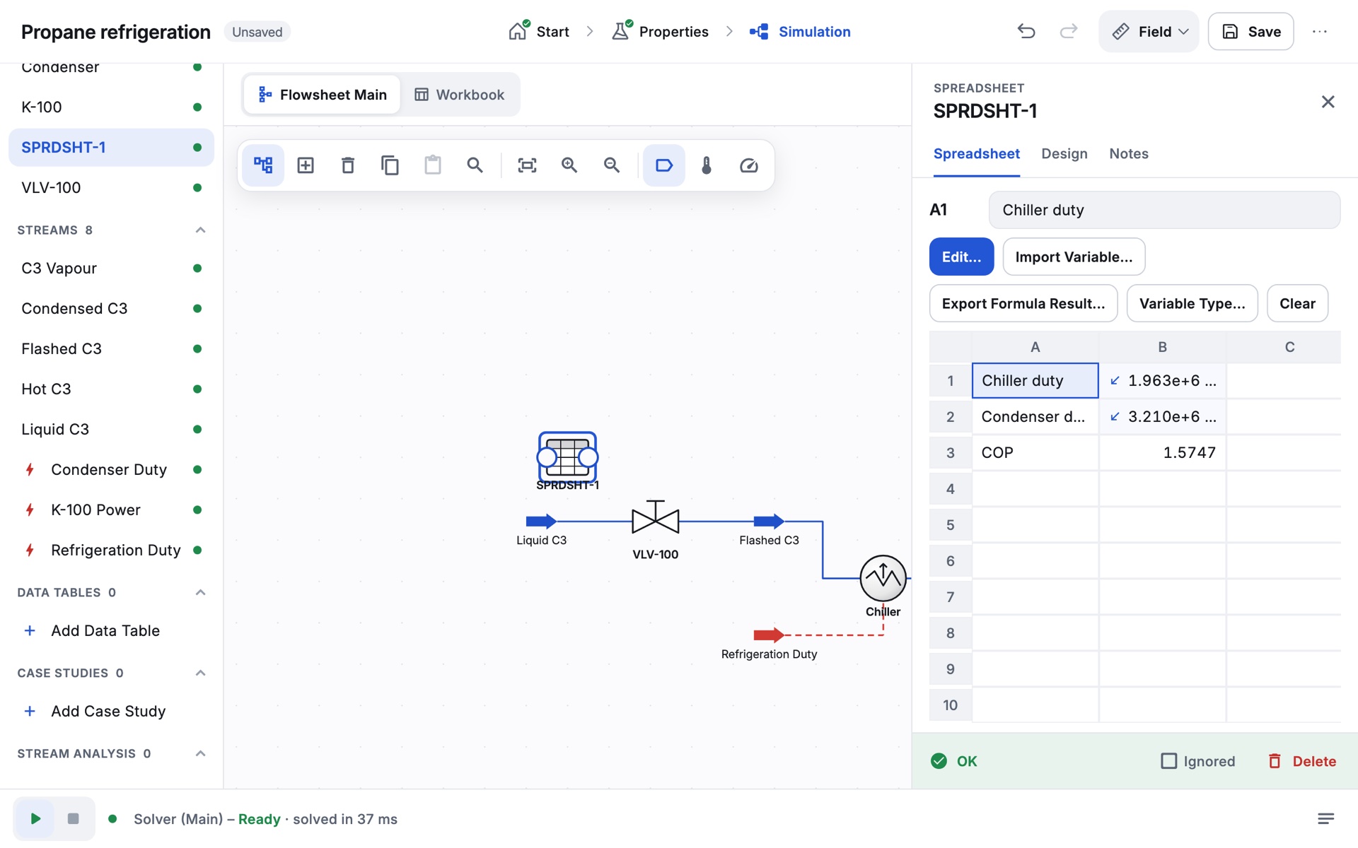
On the refrigeration loop, let cells calculate the coefficient of performance. Compressor power is not one of the variables a spreadsheet can import, but the energy balance gives it: the valve neither adds nor removes heat, so the compressor work equals the condenser duty minus the chiller duty. The COP is therefore chiller duty ÷ (condenser duty − chiller duty).
- Open Propane refrigeration from Oil & gas starter cases.
- Place a Spreadsheet from the palette. SPRDSHT-1 opens on its Spreadsheet tab.
- Type labels: tap A1 twice (or Edit...) and enter
Chiller duty; putCondenser dutyin A2 andCOPin A3. - Select B1, tap Import Variable... and pick Chiller › Duty. Import Condenser › Duty into B2.
- Select B3, tap Edit... and enter
=B1/(B2-B1).
B3 shows 1.5747, the loop's COP (1.57). Because it is a ratio of two duties, the result does not depend on the units. Change the valve pressure and the cell updates with every solve.
Case Study: sweep the chiller temperature
On the Gas plant sample, see how the liquid recovered in the low temperature separator changes with the chiller outlet temperature.
- Open Gas plant from Samples on the Start page.
- In the navigator pane, under Case Studies, tap Add Case Study.
- Tap Select a specification… and pick Chiller › Outlet Temperature (spec).
- Set Low Bound, High Bound and Step Size for the range you want to study, for example -20 °F to 20 °F in steps of 5 °F. (Up to 100 points.)
- Under DEPENDENT VARIABLES, tap Add and pick LTSLiq › Molar Flow. Add Chiller's duty too if you like.
- Tap Run, then open the Results page for the plot and the table.
The study runs on a copy of the case, so your flowsheet keeps its chiller temperature. Make sure the solver is active before you run it.